Algorithm Complexity and Big O Notation

Algorithm complexity measures how an algorithm's cost — its running time or memory usage — grows as the size of the input increases. It lets you compare algorithms independently of the machine, language or compiler: what matters is not how many milliseconds a single run took, but how fast the number of operations grows when the data gets bigger.

Asymptotic complexity and Big O notation

Asymptotic complexity describes how an algorithm behaves as the input size n approaches infinity. On small inputs even an inefficient algorithm runs fast, so what we really care about is the growth trend on large n.

This trend is expressed with Big O notation. Writing O(f(n)) means the number of operations grows no faster than the function f(n), up to a constant factor. For example, O(n) is linear growth — double the data and the time roughly doubles; O(n^2) is quadratic — double the data and the time grows four times.

Main complexity classes

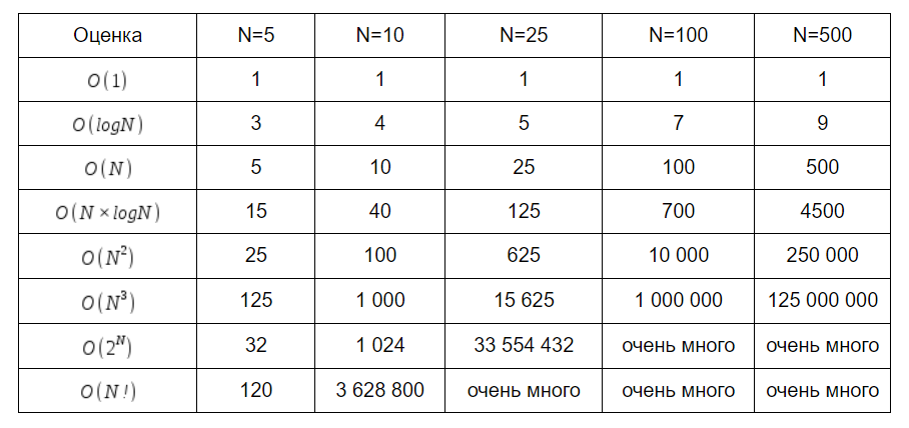
These are the classes you will meet most often (listed from fastest to slowest):

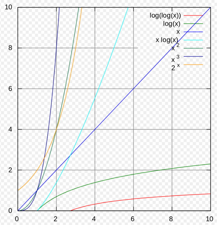
The difference in growth rate is easiest to see on a chart: the steeper the curve, the worse the algorithm scales.

Java examples by class

O(1) — constant. The number of operations does not depend on the array size: indexing takes a single step.

int first(int[] arr) {
    return arr[0]; // one operation regardless of array length
}

O(n) — linear. A single loop over every element: the bigger the array, the more iterations.

int sum(int[] arr) {
    int total = 0;
    for (int value : arr) { // n iterations
        total += value;
    }
    return total;
}

O(log n) — logarithmic. Binary search discards half of the range on each step, so the number of steps grows like the logarithm of n.

int binarySearch(int[] sorted, int key) {
    int low = 0, high = sorted.length - 1;
    while (low <= high) {
        int mid = (low + high) / 2;
        if (sorted[mid] == key) return mid;
        if (sorted[mid] < key) low = mid + 1;
        else high = mid - 1;
    }
    return -1;
}

O(n log n) — quasilinear. This is the complexity of efficient sorts. In Java you simply call Arrays.sort:

int[] data = {5, 2, 8, 1, 9};
java.util.Arrays.sort(data); // sorts in O(n log n)

O(n^2) — quadratic. A nested loop: for each of the n elements it does another n steps.

void printPairs(int[] arr) {
    for (int i = 0; i < arr.length; i++) {        // n times
        for (int j = 0; j < arr.length; j++) {    // and n more times
            System.out.println(arr[i] + ", " + arr[j]);
        }
    }
}

O(2^n) — exponential. Naive recursive Fibonacci spawns two calls every step, so the number of operations doubles as n grows.

long fib(int n) {
    if (n < 2) return n;
    return fib(n - 1) + fib(n - 2); // two calls per step
}

Rules for calculating Big O

To reduce an expression to Big O notation, apply a few rules:

• Constant multipliers are dropped — they do not affect the order of growth:

  8n^4 = O(n^4),   (n^2)/5 = O(n^2)

• Only the fastest-growing term counts — for large n the other terms become negligible:

  n^2 + n = O(n^2),   2^n + n^9 = O(2^n)

• The logarithm base is omitted: logarithms with different bases differ only by a constant factor, so we just write O(log n).

• Sequential blocks add up, nested blocks multiply. Two loops in a row give O(n) + O(n) = O(n), while a loop inside a loop gives O(n) × O(n) = O(n^2).

Time and space complexity

Complexity is measured against two resources:

• Time complexity — how the number of operations (and therefore the running time) grows.
• Space complexity — how much extra memory the algorithm uses in addition to the input itself.

The two do not have to match. An algorithm can run in O(n) time yet need only O(1) extra memory (walking an array while keeping just a counter). Often you trade one for the other: caching results to save time increases memory usage.

Worst, average and best case

The same algorithm can behave differently depending on the input, so three estimates are distinguished:

• Worst case — the upper bound, denoted with Big O. It is the one usually quoted because it guarantees the algorithm will be no slower than that.
• Average case — typical behaviour on random input (Theta, "Big Theta").
• Best case — the lower bound (Omega, "Big Omega").

Example: linear search finds the element immediately in the best case — O(1) — but scans the whole array in the worst case — O(n). When people say "linear search is O(n)", they mean the worst case.

How to estimate complexity in practice

A quick rule of thumb for eyeballing code:

• No loops, only simple operations and index access — O(1).
• A single loop over the data — O(n).
• A loop inside a loop over the same data — O(n^2); three nested loops — O(n^3).
• The range is halved on each step (binary search, walking a balanced tree) — O(log n).
• A loop that halves the data inside it, or an efficient sort — O(n log n).
• Recursion that spawns several calls over almost the same amount of data on each step — often O(2^n).

Where developers get tripped up

• Treating Big O as exact time. It is an order of growth, not a number of seconds; constants are deliberately dropped.
• Assuming O(1) means "instant". It means "independent of input size", but the operation itself can still be heavy.
• Missing hidden loops. A call like list.contains(x) inside a loop adds another O(n), turning a pass into O(n^2).
• Confusing the complexity of a data structure with that of an operation. On ArrayList, index access is O(1) but inserting at the front is O(n); on HashMap, lookup is O(1) on average but can degrade in the worst case.